Making big cat states using even-parity projectors
Author: Guillaume Thekkadath
In this tutorial, we numerically simulate the protocol proposed in Engineering Schrödinger cat states with a photonic even-parity detector, Quantum 4, 239 (2020), for engineering superpositions of coherent states. We study how to make big cat states \(|\text{cat}\rangle \sim |\alpha \rangle + |-\alpha \rangle\) with \(|\alpha|^2 = 10\).
[1]:
import numpy as np
from qutip import wigner, Qobj, wigner_cmap

import matplotlib.pyplot as plt
import matplotlib as mpl
from matplotlib import cm

import strawberryfields as sf
from strawberryfields.ops import *
from thewalrus.quantum import state_vector, density_matrix
Ideal preparation
Here we setup some basic parameters, like the value of the photon-number-resolving detectors we will use to herald and the parameters of the different Gaussian unitaries.
[2]:
Lambda = 0.9 # Lambda is a squeezing parameter in [0,1)
r = np.arctanh(Lambda)
catSize = 10 # One obtains a better fidelity when this number is an integer (see paper for explanation)
alpha = np.sqrt(catSize)*Lambda # Coherent state amplitude is chosen to compensate finite squeezing, Lambda < 1
detOutcome = int(round(catSize))
m0 = detOutcome
m1 = detOutcome
print(m0,m1)
10 10
Now we setup a 3-mode quantum circuit in Strawberry Fields and obtain the covariance matrix and vector of means of the Gaussian state.
[3]:
nmodes = 3
prog = sf.Program(nmodes)
eng = sf.Engine("gaussian")
with prog.context as q:
    S2gate(r)             | (q[1],q[2])
    Dgate(1j*alpha)       | q[0]
    BSgate()              | (q[0],q[1])
state = eng.run(prog).state
mu = state.means()
cov = state.cov()
[4]:
# Here we use the sf circuit drawer and standard linux utilities
# to generate an svg representing the circuit
file, _ = prog.draw_circuit()
filepdf = file[0:-3]+"pdf"
filepdf = filepdf.replace("circuit_tex/","")
filecrop = filepdf.replace(".pdf","-crop.pdf")
name = "cat_circuit.svg"
!pdflatex  $file > /dev/null 2>&1
!pdfcrop $filepdf > /dev/null 2>&1
!pdf2svg $filecrop $name
Here is a graphical representation of the circuit. It is always assumed that the input is vacuum in all the modes. 
We can now inspect the covariance matrix and vector of means. Note that the vector of means is non-zero since we used a displacement gate.
[5]:
print(np.round(mu,10))
print(np.round(cov,10))
[0.         0.         0.         4.02492236 4.02492236 0.        ]
[[ 5.26315789 -4.26315789 -6.69890635  0.         -0.          0.        ]
 [-4.26315789  5.26315789  6.69890635 -0.          0.         -0.        ]
 [-6.69890635  6.69890635  9.52631579  0.         -0.          0.        ]
 [ 0.         -0.          0.          5.26315789 -4.26315789  6.69890635]
 [-0.          0.         -0.         -4.26315789  5.26315789 -6.69890635]
 [ 0.         -0.          0.          6.69890635 -6.69890635  9.52631579]]
We now use The Walrus to obtain the Fock representation of the state psi that is heralded when modes 0 and 1 are measured to have the value \(n=10\). We also calculate the probability of success in heralding in the variable p_psi.
[6]:
cutoff = 18
psi = state_vector(mu, cov, post_select={0:m0,1:m1}, normalize=False, cutoff=cutoff)
p_psi = np.linalg.norm(psi)
psi = psi/p_psi
print("The probability of successful heralding is ", np.round(p_psi**2,5))
The probability of successful heralding is 0.0006
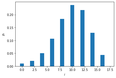
We now plot the photon-number distribution of the heralded state. Note that the state only has even photon components.
[7]:
plt.bar(np.arange(cutoff),np.abs(psi)**2)
plt.xlabel("$i$")
plt.ylabel(r"$p_i$")
plt.show()
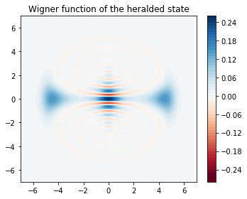
We can now plot the Wigner function of the heralded state,
[8]:
grid = 100
xvec = np.linspace(-7,7,grid)
Wp = wigner(Qobj(psi), xvec, xvec)
wmap = wigner_cmap(Wp)
sc1 = np.max(Wp)
nrm = mpl.colors.Normalize(-sc1, sc1)
fig, axes = plt.subplots(1, 1, figsize=(5, 4))
plt1 = axes.contourf(xvec, xvec, Wp, 60,  cmap=cm.RdBu, norm=nrm)
axes.contour(xvec, xvec, Wp, 60,  cmap=cm.RdBu, norm=nrm)
axes.set_title("Wigner function of the heralded state");
cb1 = fig.colorbar(plt1, ax=axes)
fig.tight_layout()
plt.show()
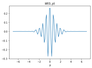
and a cut of the Wigner function along \(p=0\).
[9]:
plt.plot(xvec, Wp[:,grid//2])
plt.title(r"$W(0,p)$")
plt.xlabel(r"p")
plt.show()
[10]:
%reload_ext version_information
%version_information qutip, strawberryfields, thewalrus
[10]:
| Software | Version |
|---|---|
| Python | 3.7.5 64bit [GCC 7.3.0] |
| IPython | 7.10.1 |
| OS | Linux 4.15.0 72 generic x86_64 with debian stretch sid |
| qutip | 4.4.1 |
| strawberryfields | 0.13.0-dev |
| thewalrus | 0.11.0-dev |
| Mon Dec 30 10:15:49 2019 EST | |
Note
Click here to download this gallery page as an interactive Jupyter notebook.